Scientific visualization
Electron Orbitals
A Python visualization of electron probability density, turning radial and angular expressions into high-resolution images.
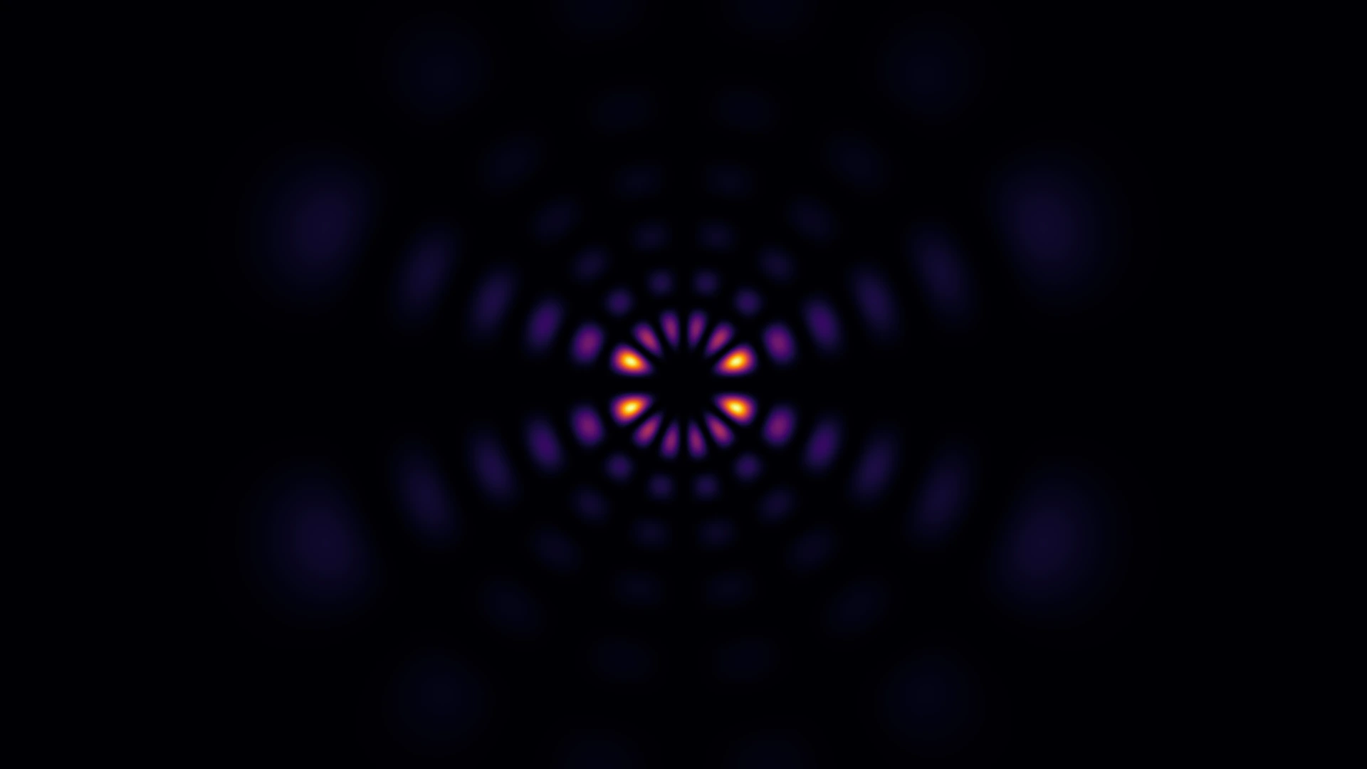
Making the calculation visible
I worked on this codebase to help my younger brother make his electron orbital visualizer more efficient. The useful change was moving symbolic work out of the per-pixel calculation: build the radial and angular expressions once, simplify them, and convert them to numerical functions with SymPy.
The renderer then evaluates those functions over a two-dimensional image. NumPy supports the numerical operations; OpenCV normalizes the result and maps it to the Inferno color palette.
From the render archive
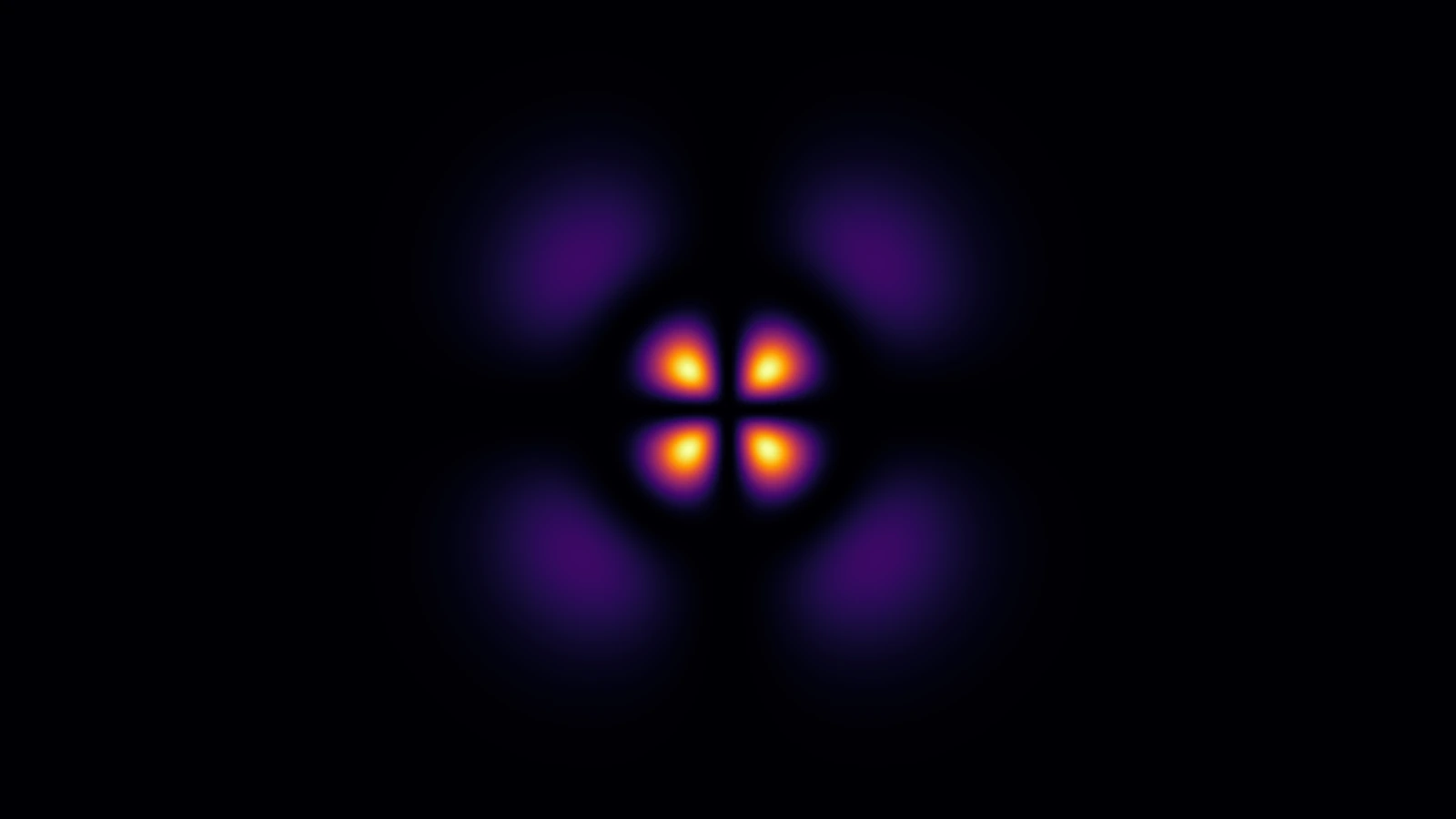
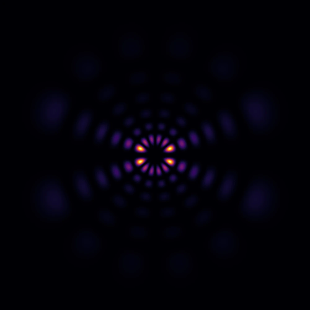
Original outputs from the Electron Orbitals repository.
Inside the implementation
- Define the state. Principal, angular, and magnetic quantum numbers parameterize associated Laguerre and Legendre expressions.
- Evaluate a plane. Image coordinates are converted to a radius and angle. The radial and angular factors are evaluated, multiplied, and squared.
- Map values to color. The field is normalized to an 8-bit image, then OpenCV’s Inferno palette makes the variation visible.
The current script uses nested Python pixel loops and requests a 7680 × 4320 render. The symbolic expressions are prepared once; the entire renderer is not vectorized. I have not measured a speedup against a baseline.
Reading these images
These are two-dimensional visualizations of a probability-density field, not paths that electrons travel. The color scale is normalized separately for each image, so brightness should not be compared as an absolute probability across renders.
The archive does not record quantum numbers for each saved image. The current script’s defaults are n = 13, l = 7, m = 2; those values should not be assumed to describe every archived render.